Author: Alexia ANGELI

There is therefore a chronological overlap between the oldest Paranthropes and the most recent Australopithecines, Australopithecus sediba having lived until 1.9 Ma, as well as with the Homo genus, which emerged around 2.8 – 2.5 Ma.

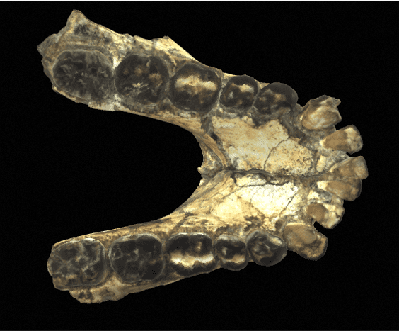
The Paranthropus genus is relatively easy to distinguish from other genera. Indeed, it is characterized by an extremely well-developed masticatory apparatus, with massive mandibles, very large premolars and molars, and very powerful masticatory muscles. In general, Paranthropes are characterized by great robustness.

A little history of science

Before going into more detail on the morphology of these 3 species, let’s take a look at the history of the Paranthropus genus. Indeed, the creation of the latter was not without its difficulties. The genus Paranthropus was first defined in 1938 by Robert Broom, following the discovery that same year of fossil remains at the Kromdaai site near Sterkfontein in South Africa. The adult male skull found was then described as Paranthropus robustus.

A few years later, in 1951, it was suggested (by Washburn and Patterson, to name but two) that the morphological differences observed between the genera Australopithecus and Paranthropus were not sufficient to justify the existence of a second genus, namely Paranthropus. A long debate within the scientific community then began on the scientific legitimacy of the genus Paranthropus.

The heart of the debate then lies in South Africa, where the Australopithecus africanus species is also present. For some scientists at the time, the particularly robust specimens (now P. robustus) were distinguished from the more graceful specimens (nowA. africanus ) also found in South Africa by a question of sexual dimorphism. So, still according to them, it’s a single species, A. africanus, with the robust individuals being the males and the more graceful individuals being the females. However, it soon becomes clear that all the gracile forms come from one and the same site, Sterkfontein, and that the same applies to the robust forms, which all come from the Swartkrans and Kromdraii sites!

What’s more, the fauna present in the Sterkfontein sedimentary fill is older and more archaic than that found at Swartkrans. This variation between the two deposits cannot therefore be the result of sexual variation, but most probably corresponds to species variation. However, some researchers decided to divide all the fossils into 2 species, Australopithecus africanus and Australopithecus robustus.

In East Africa, the first trace of Paranthropes was found in 1955 in Bed II of Olduvai (Tanzania) with the discovery of specimen OH3 (2 teeth, 1 deciduous canine and a molar) by the Leakeys. The taxonomy of this specimen remained uncertain until the 1959 discovery of a skull in Bed I of Olduvai (OH5), again by the Leakeys. For Louis Leakey, this skull differs from both Australopithecus and Paranthropus, creating a new genus, Zinjanthropus boisei. History repeats itself and in 1967, Tobias et al. consider Z. boisei to be an Australopithecus species and rename it Australopithecus boisei. The last Paranthropes species to be recognized was in 1968, under the name Paraustralopithecus aethiopicus (Arambourg and Coppens, 1968), the holotype being an adult mandible discovered in the Omo region (Ethiopia). Paraustralopithecus aethiopicus also became Australopithecus aethiopicus.

Thus, in the 1980s, the 3 current species of Paranthropes all belong to the Australopithecus genus. The name Paranthropus eventually came back into fashion following cladistic analyses demonstrating the monophyly (= 1 common ancestor) of the group formed by A. boisei, A. aethiopicus and A. robustus. It therefore seems more “logical” to group them together and separate them from Australopithecines. According to the principle of anteriority in nomenclature (to find out more, read this article), the name Paranthropus must be included.

Thus, A. boisei, A. aethiopicus andA. robustus are finally attached to the genus Paranthropus. Nevertheless, it should be noted that not all researchers agree with this, and some still use Australopithecus.

Morphological characteristics of Paranthropes

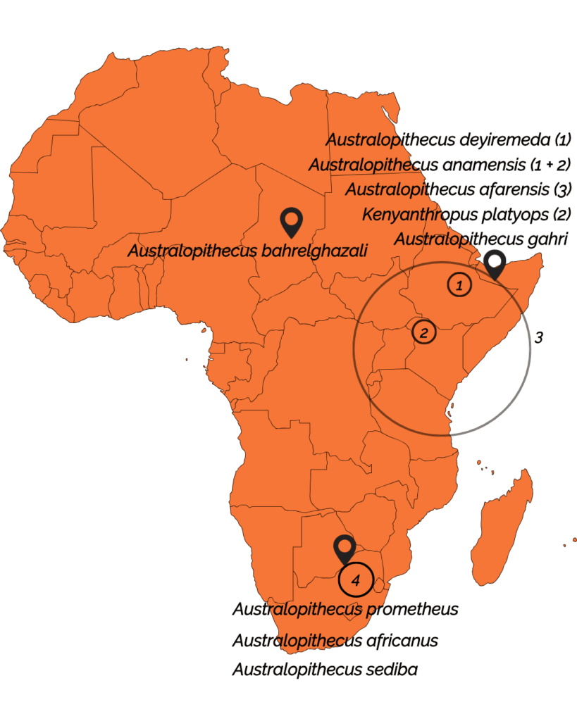
Let’s leave these epistemological debates for the moment and get back to the Paranthropes! These are classified into 3 species with different chronological extensions and geographical distributions:

• Paranthropus aethiopicus was present in East Africa between 2.98-2.87 and 2.3 Ma
• Paranthropus boisei was present in East Africa between 2.3 and 1.3 Ma
• Paranthropus robustus was present in South Africa between 2.2 and 1.2 Ma

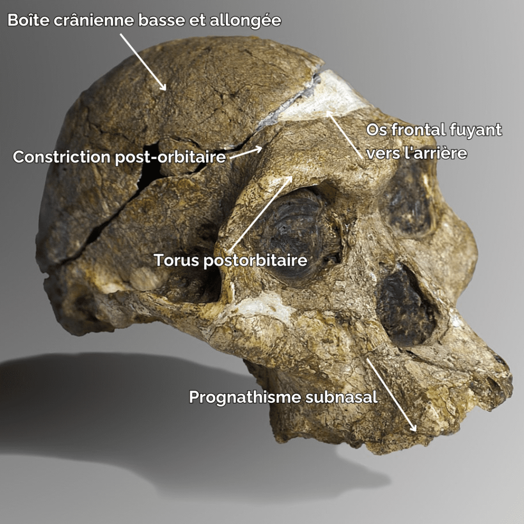
In terms of morphological characteristics, Paranthropes are characterized by extremely extensive development of the cranial superstructures. For example, males of all 3 species have a sagittal crest. The zygomatic arches are highly developed and set back from the skull. The face of Paranthropes is also wide and “hollow”, with significant alveolar prognathism, and they have no chin.

The mandibles are particularly thick and wide (much more so than in Australopithecines), and the molars are very large. Unlike Australopithecines, although they have very large premolars and molars, Paranthrope canines and incisors are small and frontally aligned. As for the skull, it features a strong post-orbital constriction (narrowing of the skull behind the orbits), a low cranial vault, a very narrow frontal bone, a cranial capacity (CC) of between 419-550 cm³ (chimpanzees have a CC of around 500 cm)³) and a thick supraorbital torus.

There are some morphological differences between the three Paranthrope species. However, the distinction between them is also based on geographical areas and chronological extension.

Locomotion & habitats

Another interesting point about Paranthropes is their type of locomotion. It is also accepted that the latter were bipedal, with more efficient bipedalism than Australopithecines, most of whom were still arboreal. Nevertheless, their bipedalism differed from our own, as Paranthropes do not have exactly the same locomotor skeleton as we do. It is also proposed that, like Australopithecines, Paranthropes may have practiced arboricolism. It should be noted, however, that the question of locomotion in this group is highly debated, as very few postcranial remains have been found.

Finally, Paranthropes lived in open (savannah-type) or closed (forest canopy) environments. Contrary to what has long been believed because of their highly-developed masticatory apparatus, Paranthropes’ diet did not consist mainly of tough foods. This belief earned P. boisei the nickname “nutcracker” (OH5). The latter was in fact only an occasional user. In reality, the Paranthropes’ diet consisted mainly of plants.

We hope you’ve enjoyed this introduction to the genus Paranthropus! Feel free to ask us questions and give us feedback on the blog. You can also contact us by e-mail. You can also follow us on Instagram, Facebook, TikTok, Twitter and YouTube!

We would like to thank paleoanthropologist François Marchal for reviewing the first version of this article.

See you soon,

The Prehistory Travel team.

Bibliography :

[1] P. Constantino, B. Wood, “Paranthropus paleobiology”, In: Miscelanea en Homenaje a Emiliano Aguirre. Volumen III: Paleoantropologia, 2004.

[2] D. Grimaud-Hervé et al.Histoire d’ancêtres. La grande aventure de la PréhistoireErrances,^5th edition, 2015.

[3] A. Rotman, “The Robust Australopithecines: evidence for the genus Paranthropus”, University of Western Ontario Journal of Anhtropology, 2011.

[4] C. Springer, P. Andrews, The complete world of Human evolution, ed. Thames & Hudson, 2011

[5] B. Wood, Wiley-Blackwell Encyclopedia of Human Evolution, Wiley-Blackwell. Reprinted edition (2013).

[6] B. Wood, P. Constantino, “Paranthropus boisei: Fifty years of Evidence and analysis”, Am. J. Phys. Anthropol. 2007

Australopithecines, what does that mean?

The term Australopithecus refers to a group of individuals that vary greatly in size and morphological conformation. In reality, Australopithecus is an informal group, as it is not monophyletic (a group with a single common ancestor) but paraphyletic (a group with several common ancestors). For this reason, they may not all belong to the same genre. In fact, one of them has been classified in the genus Kenyanthropus. Although all other species are currently classified within the Australopithecus genus, this has not yet stabilized and could change in the future. The problem lies in the extreme difficulty of diagnosing kinship links between different Australopithecus species using cladistic analyses. As a result, until such time as this fine-tuned classification of Australopithecines is obtained, which could enable some of them to be grouped into different clades, and therefore different genera, paleoanthropologists are leaving (almost) all Australopithecines within the Australopithecus genus for the sake of convenience. Nevertheless, they are fully aware of the group’s paraphilia and, therefore, of the artificiality of the genre.

The earliest Australopithecines are dated at just over 4 million years (later abbreviated to Ma) and their chronological extension extends to around 1.9 Ma. This group has lived exclusively in Africa.

A little history of science

Australopithecus is one of the longest known genera. Indeed, the first Australopithecus was discovered in 1924 (almost 100 years ago!) in South Africa by Raymond Dart. This is Taung’s child. Dart named the species Australopithecus africanus in his 1925 publication.

Subsequently, other fossil sites were discovered, again in South Africa, then, from the late 1950s, also in East Africa. Among the most important discoveries, you’ll probably be familiar with Lucy, a female australopithecine discovered by Maurice Taieb, Donald Johanson and Yves Coppens in 1974, who is related to the species Australopithecus afarensis.

At first, Taung’s child was not recognized as a human ancestor by almost all scientists for many years. It was only after the Second World War that the Australopithecus (he and other fossils discovered after him in South Africa) were consensually recognized as the most distant direct ancestors of man known at the time. Nevertheless, we now know that Australopithecines are not the ancestors ofHomo sapiens, but simply a line of Hominins.

The different species of Australopithecus

The multiplication of discoveries will lead to an explosion in the number of species. There are currently nine. Here they are:

• Australopithecus anamensis: 4.2 – 3.8 Ma (Ethiopia, Kenya)
• Australopithecus afarensis : 3.7 – 3 Ma (Ethiopia, Kenya, Tanzania)
• Australopithecus prometheus : 3.67 – 3 Ma (Sterkfontein, South Africa)
• Australopithecus deyiremeda : 3.5 – 3.3 Ma (Ethiopia)
• Kenyanthropus platyops : approx. 3.5 – 3.2 Ma (Kenya)
• Australopithecus bahrelghazali : 3.5 – 3 Ma (Chad)
• Australopithecus africanus : 3 – 2.5 Ma (South Africa)
• Australopithecus garhi : 2.5 Ma (Ethiopia)
• Australopithecus sediba : 2 Ma (South Africa)

All these specimens were mainly found in three regions:

• Gauteng province (South Africa)
• Lake Turkana Basin (East Africa)
• Awash Valley (East Africa)

The deposits in these three regions account for 95% of the fossils found in Africa, even though they correspond to very small areas on the scale of the African continent. Bear in mind, therefore, that we are working with partial and highly localized information.

What are the main anatomical features of Australopithecines?

Australopithecines have a cranial capacity of between 380 and 500 ^cm3. The skull is low and elongated. The part of the skull just behind the eye sockets is very tight; the post-orbital constriction is said to be strong. The frontal bone is narrow and tapers backwards. Above the orbits, there is a postorbital torus, i.e. a bony thickening. This varies from one Australopithecus species to another.

The face shows significant subnasal prognathism, i.e. forward projection of the face, mainly in the maxilla.

On the face, the zygomatic arches project to the sides. They are large and massive, indicating a strong masticatory force.

The mandible is massive, with a fairly high, thick mandibular body. The symphysis, where the two hemi-mandibles fuse, is more or less receding towards the back.

When it comes to teeth, there are major differences between species, as well as between males and females. Overall, you can see that molars are large. The canine teeth are smaller than those of chimpanzees, resulting in a gradual reduction in diastema (space between canine and incisor), until they disappear completely in some species.

Australopithecine modes of locomotion

The upper limbs are longer than the lower ones, but it’s difficult to say more because the species in this genus are so different in size and conformation. Nevertheless, these proportions are similar to those found in chimpanzees. This suggests that Australopithecines were still climbing trees to get around. Nevertheless, they were also capable of bipedal movement, although their bipedalism bears no resemblance to our own. To find out more about the skeletal adaptations required for bipedalism, we invite you to read this article. Australopithecines were very diverse in terms of their locomotor apparatus, and did not all use the same mode of locomotion.

We would like to thank paleoanthropologist François Marchal for reviewing the first version of this article.

We hope you find this introduction to the Australopithecus genus interesting! Feel free to ask us questions and give us feedback on the blog. You can also contact us by e-mail. You can also follow us on Instagram, Facebook, TikTok, Twitter and YouTube!

See you soon,

The Prehistory Travel team.

Bibliography :

[1] Dominique Grimaud-Hervé et al.History of ancestors. The great adventure of prehistoryErrances,^5th edition, 2015.

[2] B. Wood, Wiley-Blackwell Encyclopedia of Human Evolution, Wiley-Blackwell. Reprinted edition (2013).

Where does the term species come from?

The term species comes from Latin and means “appearance, aspect, type”. So, at first glance, a species refers to a group of individuals or objects with physical similarities. As early as 1734, Réaumur, a French physicist and naturalist, defined species as “all living beings, bodies, substances, figures or geometric shapes with similar properties” [9].

In the 18th century, European naturalists embarked on voyages across all oceans and continents, discovering hitherto unknown animals and plants. It then becomes essential for them to classify and name them. At that time, species classification was based mainly on physical criteria. These observations are therefore subject to a certain degree of subjectivity, as the perception of what is similar or different sometimes varies considerably from one observer to another. As a result, some species are given not only several names, but also different denominations in different languages.

Carl von Linné established the species as the basic heading of his classification system. In 1758, in the 10th edition of his Systema Naturae, he created the species Homo sapiens (our species) and classified it in the primate order. Linnaeus’ classification system is still in use today, although many corrections have been made to his original classification.

For Linnaeus, classification was simply a means of making the divine plan of creation intelligible, without any idea of evolution. In his view, “there are as many species as the Infinite Being produced forms in the beginning” [6]. Linné had a static vision of species, based mainly on morphological criteria.

How do you name a species?

During the 20th century, international botanical and zoological congresses sought to eliminate the confusion caused by the multiple names given to species and thus establish a nomenclature. According to this code, the name of a species is composed of the name of the genus, beginning with a capital letter, followed by the qualifier of the species, which begins with a lower case letter, followed by the initials or abbreviation of the name of its discoverer. Genus and species names are always written in italics.

ex: Homo sapiens -> Homo = genus, sapiens = species.

In addition, the principle of seniority has been established, meaning that the first name given to the species is the one that will always be retained. A species can change genus, but its name must remain.

e.g. Pithecanthropus erectus, which became Homo erectus.

Species definitions

From a classification point of view, the species represents the smallest entity, just above the individual. Nevertheless, many definitions of “this smallest entity” are proposed.

With Darwin, the static conception of the species as conceived by Linnaeus is no longer adequate. Indeed, according to Darwin and his book The Origin of Species (1859), the classification of organisms should reflect their evolutionary history.

Thus, at the end of the 19th century, the species can no longer be considered as fixed, perfectly defined, with immutable borders, existing since ever and for ever since :

– Species evolve(click here to read our article on evolution)

– More and more fossil species are being discovered- Species contours are difficult to establish in both space and time

From the twentieth century onwards, numerous definitions of the term species have emerged.

For example, in 1937, Theodosius Dobzhansky, biologist, geneticist and evolutionary theorist, was the first to propose a biological definition of species. According to him, a species corresponds to “the stage in an evolutionary process where several groups that were previously in an interbreeding relationship […] separate into at least two distinct groups, between which there can no longer be any interbreeding” [3] . Here, the term interbreeding is to be understood as interfertility. However, this definition has been criticized because it describes the mechanisms of speciation rather than what a species is in itself.

This has given rise to many other concepts of the species, such as the ecological concept of the species. This defines a species in terms of its ecological niche, i.e. the set of environmental conditions in which it lives and perpetuates itself.

In 1942, Ernst Mayr, ornithologist, biologist and geneticist, proposed a definition of biological species directly related to that proposed by Dobzhansky, and which is still taught in schools today. To do this, he relies on the criterion of interfertility. The idea is simple: if living beings can reproduce and produce fertile offspring, then they belong to the same species.

However, the definition of a species is not quite so simple. The interfertility criterion poses several problems. For example, this is not a truly operational criterion, as we can never really verify this inter-fertility, notably because of the geographical and temporal dimensions that we cannot “control”.

For example, until recently we thought that polar bears and grizzly bears couldn’t hybridize and produce fertile offspring, but that’s not the case! Indeed, due to global warming, these two species are increasingly crossing paths in the environment, and the hybrids born of these encounters (called grolars or pizzlies) are indeed fertile! Does this mean that polar bears and grizzly bears are the same species? No, this would mean wiping out thousands of years of separate evolution resulting in genetic, morphological and other differences between the two species.

Since then, other definitions have been formulated, such as the ecological species (Andersson, 1990) or the genetic species (Mallet, 1995). In 1997, R.L. Mayden listed at least 22 different concepts of species.

Why several definitions for a single “reality”?

The reason we find it so hard to agree on a single definition of species is quite simply that species does not intrinsically exist in nature. There are only notions or concepts of what a species might be. Indeed, the desire to name and categorize the world is something unique to us humans. The notion of species was therefore invented to help categorize living things into different boxes such as kingdom, order, family, etc. But in nature, there are only individuals. Whether you call the flower in your garden a “dandelion” or a “daisy” makes no difference to this individual, who will continue to exist no matter what you call him. So the concept of species is a human invention. However, nature is far more complex than simply classifying living things into distinct categories.

Living things are constantly evolving, but they also have unique intra-specific characteristics. There may also be other types of major differences within a single species, such as sexual dimorphism. For example, in great apes such as gorillas, there are significant differences between males (presence of a sagittal crest) and females (absence of a sagittal crest).

Beyond intra-species differences, it can sometimes be difficult to determine the degree of difference at which a species is considered to be different.

How can the notion of species be used in paleoanthropology?

How can we distinguish between different species on the basis of fossil remains that are often fragmentary and badly damaged? This question is still at the heart of debates within the paleoanthropology community.

When studying fossils, certain criteria cannot be verified, such as inter-fertility, which Ernst Mayr has been criticized for. As a result, morphological characteristics are most often used to define a species. This list of characters is called a “diagnose”. It is based on a fossil chosen as a reference, called the “holotype”. Nevertheless, it’s sometimes difficult to know where to draw the line when integrating or rejecting a trait for a species.

Revolutionary concepts of the species were born to alleviate this problem. This is the case, for example, of paleontologist and evolutionary systematist Georges Gaylord Simpson, who defines a species as a phyletic lineage evolving independently of others, with its own distinct and unitary evolutionary roles and tendencies.

However, evolution is a slow process, taking place over many millions of years, so the morphological traits studied don’t change all at once. It takes several thousand years for the characteristics of a species to appear and become permanently fixed in the population. A striking example isHomo neanderthalensis. In fact, the first Neanderthal-type morphological features appeared as early as around 300,000 years ago in certain populations known as pre-Neanderthals. Nevertheless, the full range of morphological features specific to Neanderthal were present around 140,000 years ago, by which time the species Homo neanderthalensis was considered to have existed. Nevertheless, should we consider pre-Neanderthal populations as already being in some way Neanderthals or as belonging to another species, Neanderthal’s ancestor?

Moreover, it’s sometimes difficult to differentiate between sexual dimorphism and morphological variation within what we consider a species, or a different species. We then subjectively choose to set limits to define species by including or excluding certain fossils, and these choices can also evolve over time.

At the end of the 20th century, Cracraft (1983) formulated the phylogenetic concept of the species in order to overcome the difficulties outlined above. According to him, the species is the smallest diagnosable group of individual organisms within which there is a parental pattern of ancestry and descent. In 1990, Nixon & Wheeler reformulated Cracraft’s definition: “the smallest aggregation of populations (sexual) or lineages (asexual) that can be diagnosed by a unique combination of character states in comparable individuals (semaphoronts = an organism as seen in a certain period of time, however brief, but not a snapshot). A character state is an attribute inherited from a common ancestor and present in all comparable individuals”.

How does paleoanthropology work in practice?

At present, the definition of the species remains as vague as ever. However, the only concept of species that can be tested and falsified is the phylogenetic concept, even though it has been much criticized for the taxonomic inflation it engenders, i.e. the creation of additional distinct species and genera.

Nevertheless, the phylogenetic concept of the species is the only one that can test and prove the existence of an evolutionary lineage.

In paleoanthropology, the specimens studied are fossils. Thus, the distinction between species is necessarily based on morphological and possibly genetic characteristics. This is part of the paleontological concept of the species.

Nevertheless, we must be careful not to mix up the different concepts, especially when trying to apply biological concepts to fossil species, such as the criterion of inter-fertility. For example, Homo sapiens and Homo neanderthalensis are two different “paleontological” species. Once again, this does not rule out the possibility of hybridization between the two species! However, to lump them together as a single species would be to overlook their separate evolutionary histories.

In conclusion, it’s important to remember that if everything has the same name, it becomes difficult, if not impossible, to study evolutionary histories. Taxonomy and classification in themselves are artificial constructs. Only phylogeny, the history of life, has a biological reality. However, to study phylogeny, it is necessary to assign names to the entities under study. At the end of the day, the name doesn’t really matter. The most important thing is to describe the people you’re talking about in such a way that everyone, whatever they call them, can understand what you’re talking about.

We hope you found this article interesting. If you have any questions or comments, we’d be delighted to hear from you. You can also contact us by email. You can also follow us on Instagram, Facebook, Twitter, TikTok and YouTube .

Bibliography :

[1] Arnould P., ” Biodiversité : la confusion des chiffres et des territoires “, Annales de géographie, vol. 651, no. 5, 2006, pp. 528-549.

[2] Buffon G., Histoire naturelle, générale et particulière. Tome II, 1749.

[3] Darwin C., On the Origin of Species by Natural Selection or the Preservation of Favored Races in the Struggle for Life, ed. orginale 1859, 2022, éditions Flammarion.

[4] Dreuil D., “Theodosius Dobzhansky”, in P. Tort (ed.), Dictionnaire du darwinisme et de l’évolution, PUF, 1996, tome 1, p. 1239-1255.

[5] Gontier T., Animal et animalité dans la philosophie de la Renaissance et de l’Age Classique, Éditions de l’Institut supérieur de philosophie, 2005.

[6] Linné C., Genera plantarum eorumque characteres naturales secundum nuemrum, figuram, situm & proportionem omnium fructificationes partiums, 1737.

[7] Linné C. Systema Naturae, 1758.

[8] Mayden R.L., “A hierarchy of species concepts: the denouement in the saga of the species”, in M. F. Claridge, H. A. Dawah, M. R. Wilson, Species: The units of diversity, London, Chapman & Hall, 1997, pp. 381-423.

[9] Réaumur, Insectes, Premier discours, Second mémoire, 1734, page 52, in Gallica

[10] Reed, et al, “Hominin nomenclature and the importance of information systems for managing complexity in paleoanthropology”, Journal of Human Evolution, vol. 175, 2023.

[11] Simpson, Wiley, Systematic Biology, Volume 27, Issue 1, March 1978, Pages 17-26, https://doi.org/10.2307/2412809

Bibliography :

Anon (n. d.) – Amazon.fr – The Big Cats and Their Fossil Relatives – An Illustrated Guide to Their Evolution and Natural History – Anton, Mauricio – Books, https://www.amazon.fr/Big-Cats-Their-Fossil-Relatives/dp/0231102291 [Accédé le 29 mars 2023].
Anon (2017) – Quaternary Extinctions, UAPress. https://uapress.arizona.edu/book/quaternary-extinctions [Accédé le 29 mars 2023].
Bargo M.S. (2001) – The ground sloth Megatherium americanum: skull shape, bite forces, and diet, Acta Palaeontologica Polonica, 46, 2.
Boeskorov G.G. (2012) – Some specific morphological and ecological features of the fossil woolly rhinoceros (Coelodonta antiquitatis Blumenbach 1799), Biology Bulletin, 39, 8, p. 692-707.
Fortin Corinne, Guillot Gérard, Le Louarn Bonnet Marie Laure, Lecointre Guillaume (2009) – Guide critique de l’évolution, Edition BELIN.
Lister A.M., Edwards C.J., Nock D. a. W., Bunce M., van Pijlen I.A., Bradley D.G., Thomas M.G., Barnes I. (2005) – The phylogenetic position of the ‘giant deer’ Megaloceros giganteus, Nature, 438, 7069, pp. 850-853.
Malhi Y., Doughty C.E., Galetti M., Smith F.A., Svenning J.-C., Terborgh J.W. (2016) – Megafauna and ecosystem function from the Pleistocene to the Anthropocene, Proceedings of the National Academy of Sciences, 113, 4, pp. 838-846.
News O.H. 10am-5pm M.-S. 10am-9pm W.C.C.D.A. 1 W.S.S.N. 2010 A.P. +61 2 9320 6000 www australian museum C.© 2023 T.A.M.A. 85 407 224 698 V.M. (n. d.) – Procoptodon goliah, The Australian Museum. https://australian.museum/learn/australia-over-time/extinct-animals/procoptodon-goliah/australian.museum/learn/australia-over-time/extinct-animals/procoptodon-goliah/ [Accédé le 29 mars 2023].
Stuart A.J., Kosintsev P.A., Higham T.F.G., Lister A.M. (2004) – Pleistocene to Holocene extinction dynamics in giant deer and woolly mammoth, Nature, 431, 7009, p. 684-689.
Stuart A. (2004) – The extinction of large mammals, Pourlascience.fr. https://www.pourlascience.fr/sd/paleontologie/https:https://www.pourlascience.fr/sd/paleontologie/l-extinction-des-grands-mammiferes-5469.php [Accédé le 4 décembre 2023].
Werdelin L., McDonald H.G., Shaw C.A. (2018) -Smilodon: The Iconic Sabertooth, JHU Press, 241 p.
Posted on Leave a comment
Australopithecines